Detecting relationships in data: Spotify Wrapped, part 4

In the first part, we talked about how to get your Spotify Wrapped data and how to visualize it. In the second part, we talked about how to process the data and how to visualize it. In the third part, we explored anomaly detection and how it helps us find interesting listening behaviour. In this part, we will talk about how to find relationships in your music.

What is a relationship?

In the context of music, a relationship can be many things. It can be the relationship between artists, genres, songs, or even the relationship between the time of day and the music you listen to. In this blog post, we will focus on the relationship between artists.

How can we explore relationships?

There is a simple solution to this and this is called Kibana Graph. Make sure that you have followed along for the data import in the second blog post, otherwise this won't work. What does Kibana Graph actually do under the hood?

Let's assume we have the following documents, each row represents a new document.

artist: ["Jamie XX"]
artist: ["Jamie XX", "Romy"]
artist: ["The XX", "Romy"]
artist: ["Jamie XX", "Fred again.."]
artist: ["Fred again..", "Romy"]

Now, Kibana Graph will compute all term co-occurrences to build the connections between each node. Therefore, we would expect a graph to look like this:

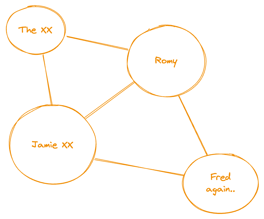
This is a very simple example, but it shows the basic idea of how Kibana Graph works. It takes all the documents and creates a graph from them. There is some terminology involved here: the circles with the artist are known as nodes or vertices and the connection between those circles is known as an edge. There are also a few tuning options that we can use:

Significant links Is a feature that helps clear out noisy terms from the dataset. This can be useful when the dataset is very noisy and documents have a large number of terms. This setting is expensive as Kibana Graph has to perform frequency checks on the Elasticsearch side for each request in order to compute the terms score, so it is recommended to turn it off if not strictly required.
Certainity By default, this is set to a value of 3, meaning the link between two artists has to appear at least 3 times in the dataset to be considered a link. I often reduce this value to 0 for other use cases, but for music, this value might be alright since I don't want to see one-time flukes in my graph. Instead, I want to see a relationship between songs I listened to more often. Turning down this value to 0 (or any other value) will increase the potential number of edges. For example, when listening once to a song that features the artists Jamie xx and Fred Again.., this is enough for the relationship to show up with a value 0. In contrast, setting it to something higher like 3 means I need to listen to the song at least 3-4 times to see a connection between those two artists.
Sample Size The graph doesn't read all documents from the index. Instead, it relies on a sample approach to create the graph. This is done to keep the performance of the graph high. We can change this number to whatever we think is representative of our dataset. However, don't forget to adjust the timeout value as you increase the sample size.
Timeout This is easy to explain. It refers to how long Elasticsearch has time to report back.

Using Kibana Graph

With the fundamentals explained, go to Kibana and click on the Graph app. You will need to select a data view, which is the Spotify History. When prompted to select a field, use the artist field. By default, that should turn out violet with a musical 16th note on it. I had to adjust my sample size to 5000 to get a good starting graph.

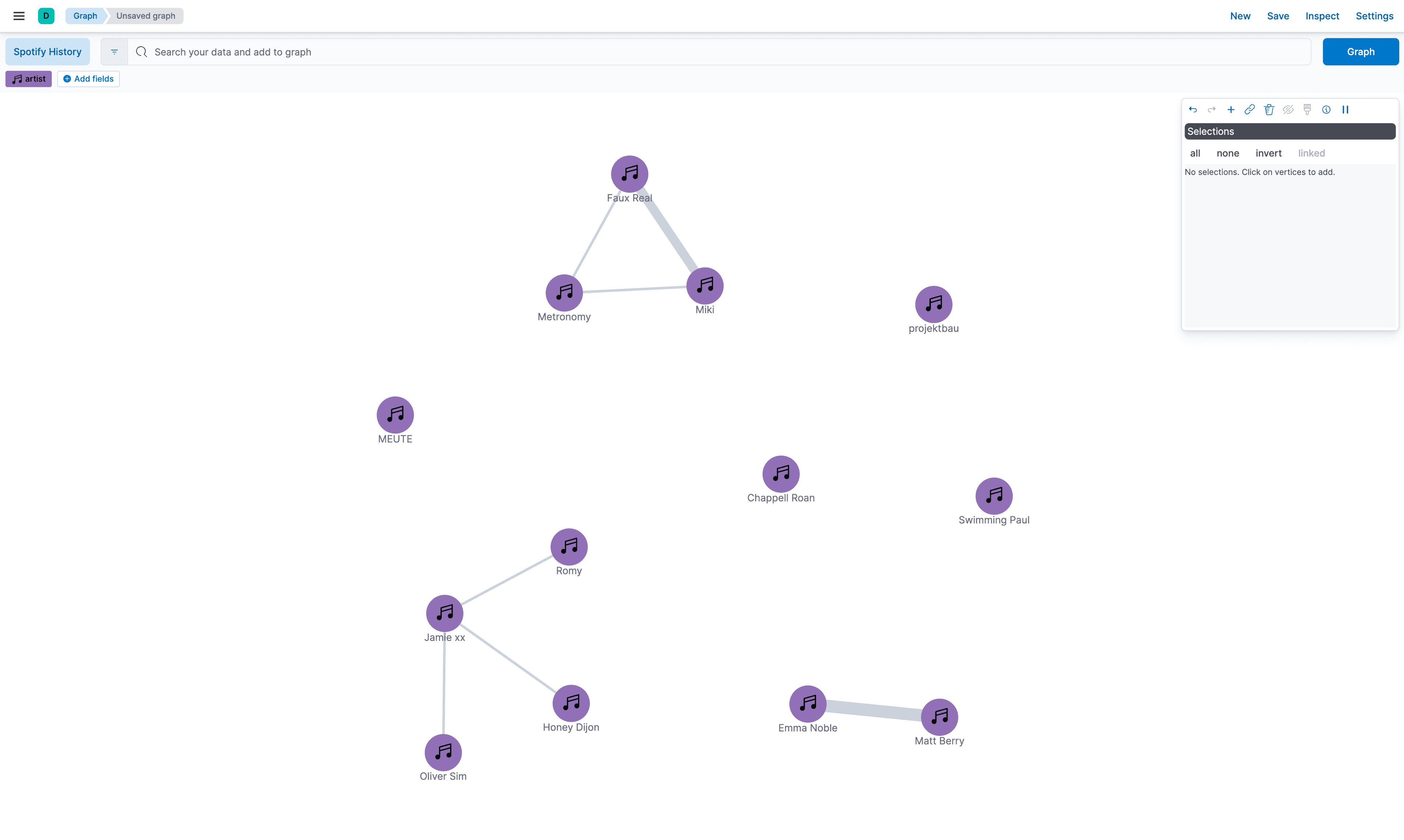
We can tell that we have multiple artists that are connected to each other. This allows us to select one of those artists and press the + sign. There are already some clusters forming, which is important. Those standalone artists are not interesting to us. There is an all button in the right panel. Select it and press the + again. This will now explode your graph and pull in the additional artists.

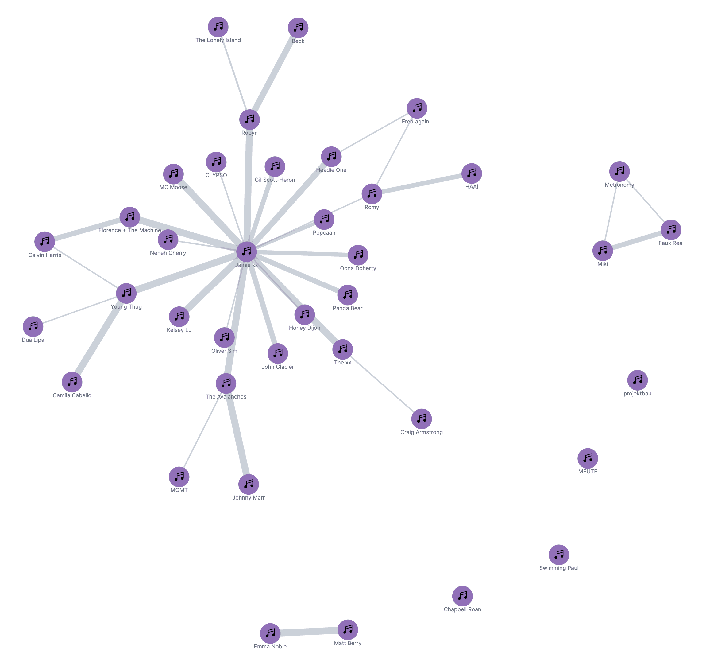
If we continue this process, increase the sample size and start exploding the graph more and more. Depending on your listening style, you should either get a lot of little islands or a few big clusters. In the next picture, we see one big cluster in the middle that interconnects Rudimental, Fred again.., and Jamie XX. This makes sense, as all of them belong to the same genre which heavily features the same artists. At the same time, we have some tinier islands around. Kraftklub is a German band and is connected to mostly all of the German music I listen to, like Casper and Blond. There are some isolated vertices such as Harry Styles.

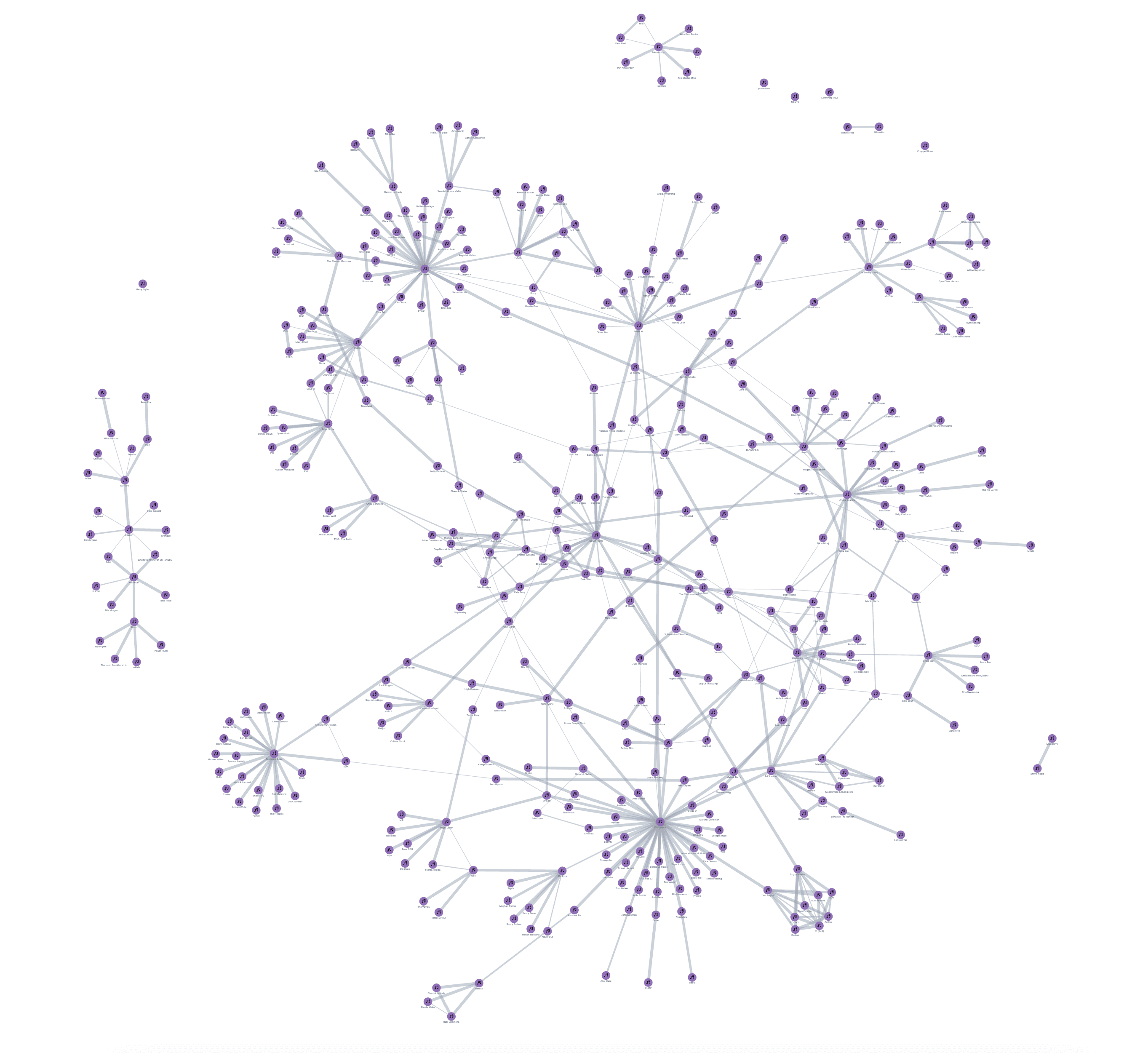
Let's dig into why Harry Styles is alone. Does he not feature anyone? How does he fit into my listening behavior when all of my other listened-to music is more or less connected based on the featuring of artists?

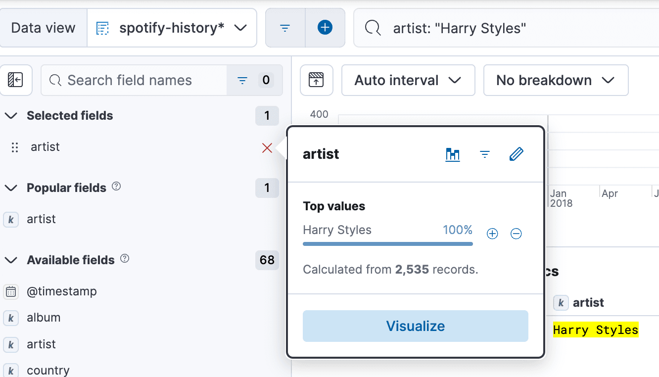
Go to Discover and perform the following:

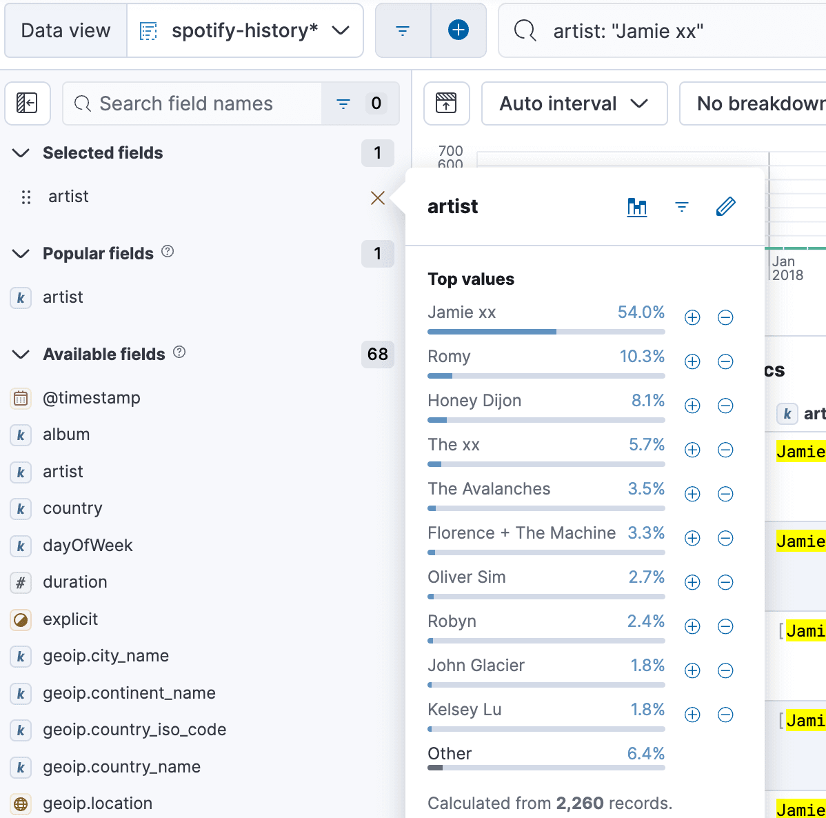
In the search bar, write artist: "Harry Styles". This filters down to all documents that have Harry Styles in the name.
We can simply click on the field artist in the field picker on the left side and see that there is only 1 value.
Even though I listened to Harry Styles 2535 times, he has never featured another artist (or at least, according to Spotify data, it is not listed as such). Compare that to e.g. Jamie XX and we can see the difference.

Conclusion

In this blog, we explored relationships and how easy it is to leverage Kibana Graph and Elasticsearch's graph capabilities. Stay tuned for more parts in this blog series!

Want to get Elastic certified? Find out when the next Elasticsearch Engineer training is running!

Elasticsearch is packed with new features to help you build the best search solutions for your use case. Dive into our sample notebooks to learn more, start a free cloud trial, or try Elastic on your local machine now.

Report an issue